While The BFD normally favors a lighter approach, with a focus on forecasting process (the politics and personalities therein), forecasting news, and forecasting gossip, we sometimes have to get serious. In this guest blogger post from Koen Knapen, Principal Consultant at SAS Belgium, Koen takes us into the netherworlds of Kalman Filtering and Kalman Smoothing. (And with the unobserved components model (PROC UCM) available in SAS/ETS® and SAS® Forecast Server, SAS will let you go as nether as you want.)
Koen Knapen on Kalman Filtering and Kalman Smoothing in SAS PROC UCM
The UCM procedure analyzes and forecasts equally spaced univariate time series data by using an unobserved components model (UCM). The UCMs are also called structural time series models in the time series literature. A UCM decomposes the response series into components such as trend, seasonals, cycles, and the regression effects due to predictor series.
You can use the OUTFOR= option in the FORECAST statement to store the series and component forecasts produced by the procedure. The OUTFOR= dataset will contain many variables (corresponding to the components) with an ‘F_’ prefix and many variables with an ‘S_’ prefix where the ‘F’ is for ‘Filtered’ (or ‘Forecasted’) and the ‘S’ is for ‘Smoothed’. With ODS GRAPHICS you can also produce time series plots of the filtered component estimates as well as time series plots of the smoothed component estimates.
Users of the UCM procedure will wonder what the difference is between the filtered and smoothed values of the components. That’s what this blog entry is about! What’s the difference between (Kalman) filtering and (Kalman) smoothing in the context of UCMs?
The UCMs considered in PROC UCM can be thought of as special cases of more general models, called (linear) Gaussian state space models (GSSM). A UCM formulated as a GSSM has essentially two equations. The first equation, called the observation equation, relates the response series y(t) to a state vector α(t) that is usually unobserved. The state vector contains the component estimates and their variance. The state vector is contained and updated in a second (recursive) equation, appropriately called the state transition equation. The state and other elements of the transition equation provide a rule for getting the model and predictions from one interval to the next. Thus the transition equation describes the evolution of the state vector in time.
The state space formulation of a UCM has many computational advantages.
In this formulation there is a convenient algorithm for estimating and forecasting the unobserved states / components (i.e. state vector α(t) at any time t) by using the observed series y(t), being the DKFS algorithm (DKFS = Diffuse Kalman Filtering and Smoothing).
The Difference between Kalman Filtering and Kalman Smoothing
So … Kalman Filtering and Kalman Smoothing: What is it and what's the difference and what is it used for?
Kalman filtering-smoothing (KFS) is a fundamental tool in statistical time-series analysis, especially in STATE SPACE MODELLING (SAS/ETS PROC SSM).
Remember … Unobserved Components Models (UCMs) can also be expressed as state space models. In SAS, UCMs (also known as Structural Time Series Models) are formulated as a state space model.
The UCM and SSM procedures use the same Kalman filtering/smoothing algorithms (despite different descriptions in their docs).
The biggest difference between Kalman filtering and Kalman smoothing is that in Kalman filtering the recursive state estimation moves forward through the data and in Kalman smoothing the recursive state estimation moves backward through the data (in the opposite direction of the time variable).
Kalman filtering is a forward pass through the data. Kalman smoothing ADDS a backward pass through the data. Smoothing is thus an add-on to filtering.
Kalman filtering uses all the data up to the current time point and can be done in real-time (given data so far).
Kalman smoothing is offline post-processing and uses all the data.
Kalman filtering has two steps: prediction at the current observation using all prior observations followed by update/filtering using the actual current observation.
If your only goal would be forecasting of the response variable Y and the state vector, Kalman filtering is sufficient.
Good reasons for Kalman smoothing are:
• The Kalman smoother provides very good imputations (i.e. imputed values) for missing values in your time series.
• The Kalman smoother provides very good estimates of the state vector in the historical period. The state vector is estimated for every historical time bucket ‘t’ and contains the component estimates and their variance. The damping factor (and other parameters such as cycle period, disturbance variances) are estimated by likelihood optimization.
• The smoothing gives full-sample versions of the historical state vectors (since all collected data are used).
• The smoothing gives a good estimate of the covariance matrix of the state variables.
• Kalman smoothers can extrapolate in a consistent fashion.
• The smoothing pass provides diagnostics for structural breaks (smoothing-based structural break diagnostics).
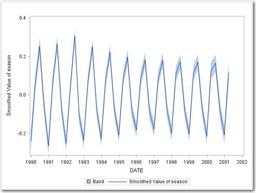
• Smoothed estimates of component values (trend, seasons, cycles, regressor effects …) can be really useful for visualization and comprehension.
For the response variable (Y), the smoothed estimates are identical to the actual values where they are non-missing.
In the PROC UCM output dataset, the component F_* and VF_* variables are coming from the filtering, the component S_* and VS_* variables are coming from the additional smoothing step. (The V is for Variance).
Where to Learn More
• Modeling Trend, Cycles, and Seasonality in Time Series Data Using PROC UCM - LWBARS/BARS course notes from SAS Institute
• Forecasting with Unobserved Components Time Series Models
Andrew Harvey, Faculty of Economics, University of Cambridge
Prepared for Handbook of Economic Forecasting (Chapter 07), 2006
• Time Series Modelling with Unobserved Components, The blog to the book, Matteo M. Pelagatti, http://www.ucmbook.info/
Good luck with your PROC UCM analyses!